This project is the first challenge of the Artificial Neural Networks and Deep Learning course at Politecnico di Milano: classifying multivariate sequences of 160 time steps into three pain levels, with one class alone covering more than three quarters of the data. The team reached 95.5% F1 on the Kaggle leaderboard, and the v2 model, whose architecture I developed, achieves a mean weighted F1 in 5-fold cross-validation of 0.9485 ± 0.0136.
Context
The challenge ran as the course's Kaggle competition in the 2025/26 academic year. I worked on it in a team with other colleagues.
To compare two set-ups, the team built two versions of the notebook: a simpler v1, with a bidirectional LSTM, an attention mechanism and Monte Carlo cross-validation, and a more elaborate v2. My contribution: I developed the v2 model architecture and added class weighting to the loss, with almost identical weights in both v1 and v2, as well as label smoothing, used in v2 only. Other parts of the work, such as the initial notebook structure, v1's Monte Carlo cross-validation and attention, v1's data augmentation (jittering) and the hyperparameter tuning, were handled by other members of the team.
Data
The challenge dataset, called the "Pirate Pain Dataset", contains 661 training sequences, each 160 time steps long. Every step records 31 joint angles (continuous values), 4 pain surveys (taking the values 0, 1 or 2) and 3 subject characteristics (n_legs, n_hands, n_eyes). The competition test set holds 1,324 unlabelled sequences.
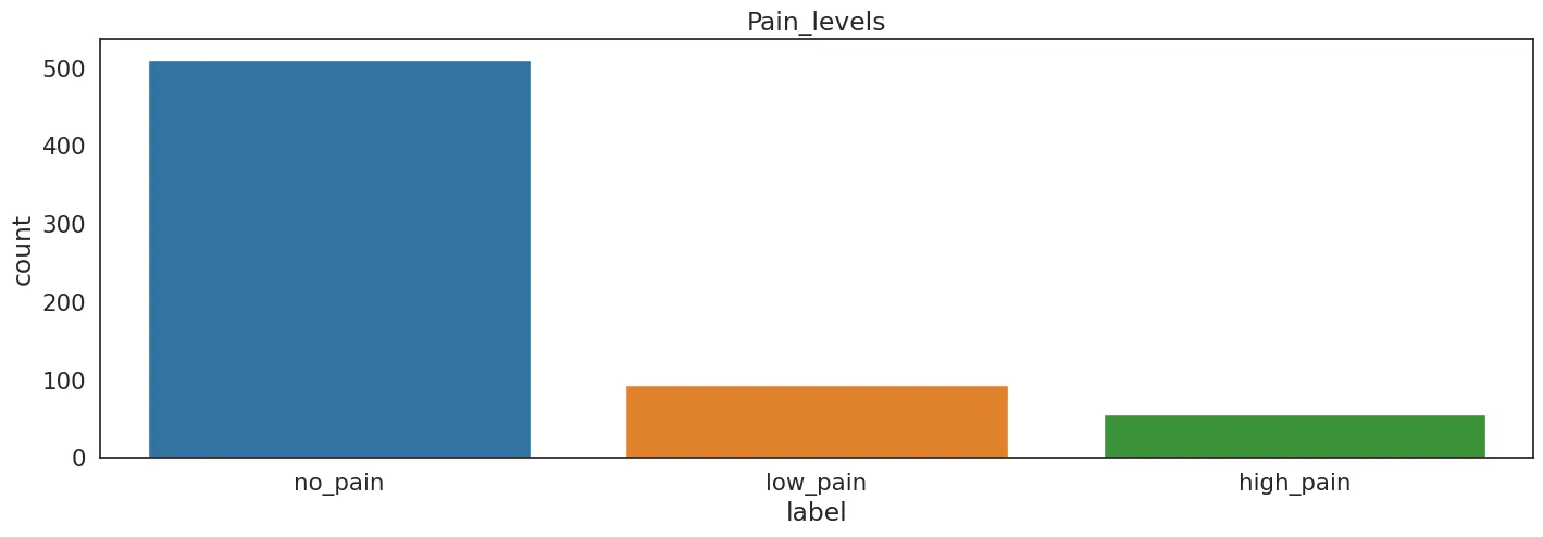
There are three labels: no_pain, low_pain and high_pain. The class distribution is heavily skewed (511 no_pain sequences, about 77.3%; 94 low_pain, 14.2%; 56 high_pain, 8.5%), and this imbalance is the main difficulty of the problem.
Exploratory analysis flagged columns to discard. joint_30 has the same value in every row and carries no information; n_legs, n_hands and n_eyes are perfectly correlated, so one of them is enough. In v2, each time step is therefore described by 30 joint angles, 5 categorical variables (n_legs and the four surveys) and the time index.
The v2 model
Windows and majority vote
Each sequence is cut into overlapping windows of 40 steps with a stride of 10, so a 160-step sequence yields 13 windows; each window inherits the label of its parent sequence. At inference time, a sequence gets the class chosen by the majority of its windows.
Architecture
The architecture I developed takes windows of 40 steps × 36 variables and handles the two kinds of input separately:
- Embeddings for the categorical variables.
n_legsand each of the four surveys go through their own embedding of size 4, instead of entering the network as ordinal numbers. Concatenated, they give 20 values per step. - Conv1D extractor on the joint angles. Two 1D convolutional layers with 128 filters and kernel size 7, each followed by ReLU and dropout 0.2, work only on the 30 joint channels to extract local patterns. Padding keeps the window length unchanged.
- GRU. At each step, the convolution output (128 values), the embeddings (20) and the time index (1) form a 149-value vector. A 2-layer unidirectional GRU with 128 hidden units and dropout 0.2 between the layers processes it.
- Attention pooling. A linear layer scores each step of the GRU output; after a softmax over time, the weighted sum of the states becomes the context vector.
- Classification head. A linear layer maps the 128-value context vector to the 3 classes.
The v1 notebook also used an attention mechanism, developed within the team; in v2, each step's score comes from a single linear layer. The code can swap the GRU for an LSTM or a plain RNN; the configuration saved in the notebook uses the GRU.
Loss and training
The loss is cross-entropy, with two changes I introduced:
- Class weighting, to counter the imbalance, with weights 0.915, 2.142 and 2.740 for
no_pain,low_painandhigh_pain: mistakes on the rare classes weigh more in the loss. They are almost identical to the weights already used in v1. - Label smoothing with ε = 0.10, in v2 only: the target is no longer a hard one-hot vector, which discourages overconfident predictions.
The rest of the v2 set-up: AdamW optimiser with learning rate 0.001 and weight decay 0.3, gradient clipping at a maximum norm of 10, a ReduceLROnPlateau scheduler on validation F1 (factor 0.5, patience 20), batches of 512 windows and up to 300 epochs, with early stopping after 100 epochs without improvement and the best weights restored. On GPU, training uses mixed precision.
Validation and ensemble
Before cross-validation, 7 sequences (about 1%) are held out as a local test set: with so few examples, the score on it would not be a reliable estimate, so I do not report it. Stratified 5-fold cross-validation runs on the remaining 654 sequences, with 131 or 130 validation sequences per fold, and assigns sequences, not windows, to the folds: the split happens before windowing, so all the windows of a sequence are either in training or in validation. Min-max normalisation of the joint angles is also fitted fold by fold, on the training part only. Each fold's score is the sequence-level weighted F1, after the majority vote over windows.
On the test set, the five fold models work together: each one votes a class for every sequence, and the votes are summed with weights proportional to the fold's validation F1.
Results
On the Kaggle leaderboard, the team reached 95.5% F1.
In cross-validation, the v2 model scores as follows, measured at sequence level on each validation fold:
| Fold | Weighted F1 | Accuracy |
|---|---|---|
| 1 | 0.9680 | 0.9695 |
| 2 | 0.9545 | 0.9542 |
| 3 | 0.9283 | 0.9313 |
| 4 | 0.9528 | 0.9542 |
| 5 | 0.9391 | 0.9385 |
| Mean ± std. dev. | 0.9485 ± 0.0136 | 0.9495 ± 0.0134 |
The whole five-fold cross-validation run took 14 minutes 50 seconds on a Google Colab GPU.
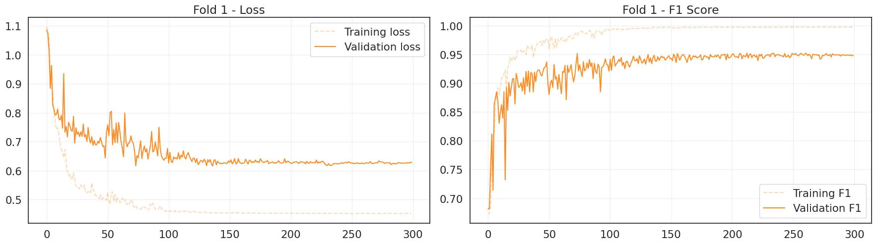
The chart at the top shows the fold-1 curves: training F1 gets close to 1, while validation F1, computed on individual windows, levels off around 0.95. The checkpoint restored at the end is the one from epoch 261.
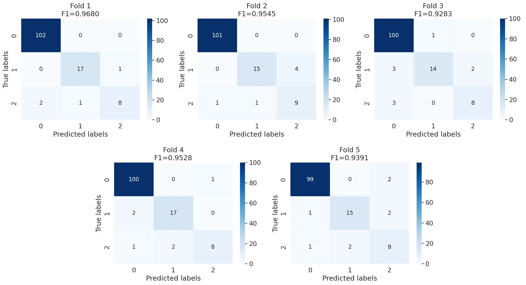
Adding up the five matrices (654 sequences), high_pain is the hardest class: 41 of 55 sequences are classified correctly, against 78 of 93 for low_pain and 502 of 506 for no_pain. The project README points to the same weakness: despite class weighting, high_pain remained the hardest class to recognise.
Limitations
- Metric. Weighted F1 weighs each class by its frequency, so it is dominated by
no_pain. For the minority classes, the confusion matrices say more. - Variability across folds. Per-fold F1 ranges from 0.9283 to 0.9680, and the best epoch from 25 to 261.
- Ensemble. The fold weights are almost equal, between 0.1957 and 0.2041: three agreeing votes always outweigh two, so the weights only matter in 2-2 ties.
- Time index. The joint angles are min-max normalised, while the time index (0 to 159) enters the network unscaled.
- Comparison with v1. In v1, the validation windows came from sequences that were also used for training, so its validation scores are optimistic and not comparable with v2's. That is why I only report v2 numbers here.
The code is public on GitHub, with the README and the v1 and v2 notebooks: github.com/devisnsk/an2dl-c1-2025. The dataset files are not included in the repository.