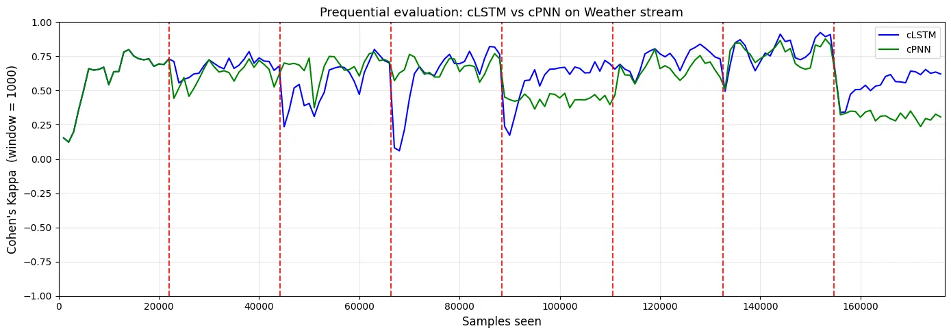
I integrated two streaming continual learning architectures, Continuous LSTM (cLSTM) and Continuous Progressive Neural Networks (cPNN), as classifiers compatible with CapyMOA, an open-source framework for learning from data streams. On the Weather stream, which goes through seven real, abrupt concept drifts, cPNN limited the collapse after several drifts and fluctuated less in most concepts, while cLSTM reached the higher mean Kappa in five of the eight concepts.
Context
This was optional project no. 7 of the Streaming Data Analytics course at Politecnico di Milano (academic year 2025/26, Prof. Emanuele Della Valle), which I carried out on my own in May 2026, starting from the course's assignment.
The subject is streaming continual learning (SCL), which the assignment presents as a synthesis of two research areas: streaming machine learning, which puts fast adaptation to concept drift first even at the cost of forgetting, and continual learning, which protects existing knowledge but was designed for concepts that do not contradict each other. On top of that, in a stream a data point is often correlated with the ones before it.
cLSTM accounts for this temporal dependence by continuously training an LSTM on sliding windows. cPNN uses it as a building block: for every new concept it adds a cLSTM "column" laterally connected to the previous one, which is frozen. The task was to bring both models into CapyMOA as classifiers, starting from the MagicNet reference implementation, and to compare them with a prequential evaluation.
Data
The Weather stream, provided by the course, has 176,844 samples with four meteorological features that are already standardised (relative humidity, dew point temperature, wind speed and wind direction) and a binary label derived from the air temperature, which is not one of the features.
The stream goes through eight concepts of about 22,100 samples each, and every concept corresponds to a labelling rule. The seven drifts are real and abrupt, and the new rule may even invert the labels of the previous one.
A task column holds the current concept: as the assignment allows, I use it to add columns to cPNN, so the drift point is known rather than estimated by a detector. The data is course material and is not included in the repository.
Approach
cLSTM as a CapyMOA classifier
CapyMOA works one instance at a time (for every new feature vector the classifier predicts, then learns from its label), whereas an LSTM works on sequences. In my subclass of capymoa.base.Classifier I bridged the gap with two mechanisms.
- Anytime inference. The classifier keeps the last W = 11 vectors and, at every sample, predicts from the last step of the window. Until it has seen 11 samples it pads the left of the window with zeros, so it can predict from the very first one; the reference implementation, by contrast, returns nothing until it has seen enough.
- Periodic training. Labelled pairs accumulate in a buffer of B = 128. When it is full, a sliding window turns it into 128 − 11 + 1 = 118 sequences, each labelled with its last sample; then come 10 epochs of Adam, and the buffer is cleared.
The underlying network, cLSTMLinear (a one-layer LSTM with a linear head), is taken from MagicNet; I reused it as is, adding only documentation. W, B, E, H and the learning rate come from the assignment; the optimiser and the loss are not specified there: I chose Adam and cross-entropy, the same ones used by the reference implementation.
| Hyperparameter | Value |
|---|---|
| Window W | 11 |
| Mini-batch B | 128 |
| Epochs per mini-batch E | 10 |
| LSTM hidden size H | 50 |
| Learning rate | 0.01 |
| Optimiser and loss | Adam, cross-entropy |
| Seed | 1 |
cPNN: one column per concept
cPNN starts with a single column, identical to cLSTM. At each drift the notebook calls add_new_column(), which freezes the active column (requires_grad = False), appends a new column with its own Adam optimiser and clears the buffer, so the new column learns only from post-drift data. Its input is the 4 features concatenated with the hidden-state sequence of the previous column: 54 values per step.
During training every column runs its forward pass, because the lateral signal has to travel through the whole chain, but only the active column updates its weights. The inference window is shared across columns, so a freshly added column does not start again from a window of zeros.
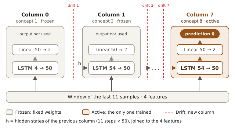
cPNN after the seven drifts: every column receives the input window and, from the second one on, the hidden states of the previous one, but only the last is trained and produces the prediction. Diagram derived from the code in cpnn.py.
By the end of the stream there are 8 columns. Computing the parameters from the layer sizes (the notebook does not report them) gives 160,416, of which only the last column's 21,302 are still trainable; cLSTM has 11,302.
Prequential evaluation
The notebook walks through the 176,844 samples one by one: it asks both models for a prediction, updates the evaluators, adds a column to cPNN if task has changed, and finally trains both models on the sample. cLSTM gets no drift signal at all, and its mini-batches can straddle the boundary between two concepts. The assignment asks for a rolling Cohen's Kappa without fixing the window size: I computed it over windows of 1,000 samples with CapyMOA's ClassificationWindowedEvaluator. All results below come from a single run with seed 1.
Results
The chart at the top shows Kappa along the whole stream. The notebook summarises the windows by concept. Mean Kappa, with the higher value in bold:
| Concept | Samples | cLSTM | cPNN | Δ (cPNN − cLSTM) |
|---|---|---|---|---|
| 1 | 0–22,095 | 0.596 | 0.596 | 0.000 |
| 2 | 22,095–44,200 | 0.678 | 0.617 | −0.061 |
| 3 | 44,200–66,305 | 0.560 | 0.679 | +0.119 |
| 4 | 66,305–88,412 | 0.613 | 0.667 | +0.054 |
| 5 | 88,412–110,520 | 0.580 | 0.436 | −0.144 |
| 6 | 110,520–132,628 | 0.732 | 0.652 | −0.080 |
| 7 | 132,628–154,736 | 0.791 | 0.766 | −0.025 |
| 8 | 154,736–176,844 | 0.556 | 0.326 | −0.230 |
Minimum and standard deviation, with the higher minimum and the lower deviation in bold:
| Concept | cLSTM min | cPNN min | cLSTM std | cPNN std |
|---|---|---|---|---|
| 1 | 0.123 | 0.123 | 0.198 | 0.198 |
| 2 | 0.556 | 0.442 | 0.055 | 0.080 |
| 3 | 0.235 | 0.375 | 0.154 | 0.085 |
| 4 | 0.060 | 0.561 | 0.214 | 0.060 |
| 5 | 0.173 | 0.364 | 0.148 | 0.032 |
| 6 | 0.552 | 0.466 | 0.072 | 0.072 |
| 7 | 0.495 | 0.510 | 0.102 | 0.086 |
| 8 | 0.340 | 0.237 | 0.086 | 0.069 |
- Concept 1. Identical results: cPNN still has a single column, with cLSTM's architecture and seed.
- Where cPNN wins. Higher mean Kappa in concepts 3 (+0.119) and 4 (+0.054). In concept 4 cLSTM drops to 0.060, while cPNN never goes below 0.561.
- Where cLSTM wins. Higher mean Kappa in concepts 2, 5, 6, 7 and 8, with the widest gaps in concept 8 (0.556 against 0.326) and concept 5 (0.580 against 0.436).
- Stability. cPNN's standard deviation is lower in concepts 3, 4, 5, 7 and 8, equal in concept 6 and higher in concept 2.
- Average over the eight concepts. Computed from the table, not by the notebook: 0.638 for cLSTM and 0.592 for cPNN.
In the notebook I wrote that cLSTM drops more than cPNN after every drift. The numbers confirm it for several drifts, not all of them: cLSTM's sharpest collapses follow the drifts into concepts 3, 4 and 5, whereas after the first drift, into concept 2, it is cPNN that drops further. In concepts 6 and 8 cPNN's minimum is also lower than cLSTM's, and in concept 7 the two minima are close (0.510 and 0.495).
How I read the comparison
It is a trade-off between plasticity and stability. cLSTM retrains all of its weights on the current concept: with a contradictory drift it first has to "unlearn" the old concept, hence the deep dips, but given enough samples it specialises and tends to overtake cPNN. In cPNN the new column starts from fresh weights, so the dips are shallower; however, it has to reconcile the new concept with the fixed lateral signal of the frozen columns, which after a contradictory drift can push it the wrong way. The result is a lower plateau, clearly visible in concepts 5 and 8.
After the run: partial mini-batches
On 28 May 2026, after the run reported here, I gave both classifiers a flush() method that trains the model on the incomplete mini-batch left in the buffer, provided it holds at least 11 samples. Until then that data was lost: in cPNN at every drift, when add_new_column() cleared the buffer, and in both models at the end of the stream, because CapyMOA does not tell classifiers that the stream has ended. Now add_new_column() calls flush() before freezing the active column, and the notebook calls it after the loop. By my count from the concept lengths (not reported in the notebook), before the change cPNN left 716 samples unused and cLSTM 76.
The results saved in the notebook come from the earlier run: for cLSTM the final flush() happens after the last evaluation and does not change the curves, whereas for cPNN the numbers on this page do not reflect the change.
Limitations
- A single run. One seed, one data file, no repetitions and no significance tests.
- Known drift points. The change points come from the
taskcolumn, not from a detector. - A single metric. Only windowed prequential Kappa, without forgetting measures, as the assignment allows.
- Approximate per-concept statistics. A window that contains a drift is assigned to the following concept.
- Unused labels. Each mini-batch is split into sequences on its own, so its first 10 labels never become training targets; in its many-to-one variant, the reference implementation instead prepends the last 10 samples of the previous batch.
- Reproducibility. The code and dependencies (
requirements.txt,uv.lock) are in the repository; the data is not.
The code for both classifiers and the notebook with the analysis are in the project repository on GitHub.